FP Growth Algorithm Explained With Numerical Example

The FP Growth algorithm is a frequent pattern mining algorithm used in market basket analysis. This article discusses the FP growth algorithm with a step-by-step numerical example.

What is the FP Growth Algorithm?

Like the apriori algorithm, the FP-Growth algorithm is also used for frequent pattern mining. The FP-Growth or Frequent Pattern Growth algorithm is an advancement to the apriori algorithm. While using the apriori algorithm for association rule mining, we need to scan the transaction dataset multiple times.  In the FP growth algorithm, we just need to scan the dataset twice.

Apart from that, we also don’t need to generate candidate sets while generating the frequent itemsets as discussed in this article on apriori algorithm numerical example. We create an FP-Tree and use it to determine the frequent itemsets. Thus, the FP-Growth algorithm helps us perform frequent pattern mining with less computing resources and even lesser time. 

What is an FP-Tree in FP Growth Algorithm?

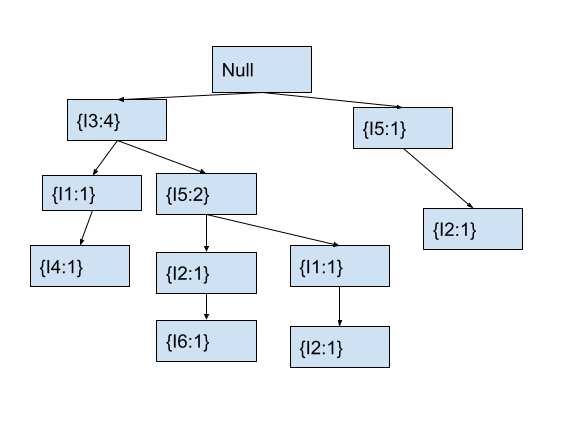
An FP-Tree is a tree data structure created from the transaction data while generating frequent itemsets in the FP growth algorithm. To create an FP-Tree, we first scan the transaction dataset and record the support count of each item. Then, we create a tree structure where each node in the tree represents an item in the dataset and its frequency count. The root node has no associated item and is used as a starting point for the tree. We denote the root node by None or Null. The children of a node in the fp-tree represent the items that frequently co-occur with the parent item in the dataset.

To construct the tree efficiently, we first transform the dataset by sorting the items in each transaction based on their support count. We do this to make sure that the frequent items appear early in each transaction. This leads to more frequent items being near the root node resulting in a compact and efficient tree. For example, consider the following dataset.

Transaction ID	Items
T1	I1, I3, I4
T2	I2, I3, I5, I6
T3	I1, I2, I3, I5
T4	I2, I5
T5	I1, I3, I5

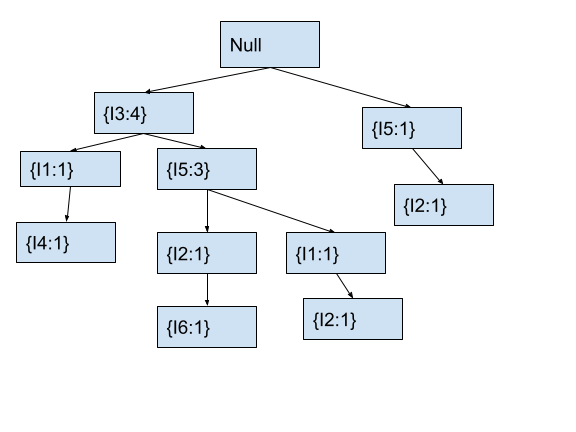
The fp-tree for the above dataset looks as follows.

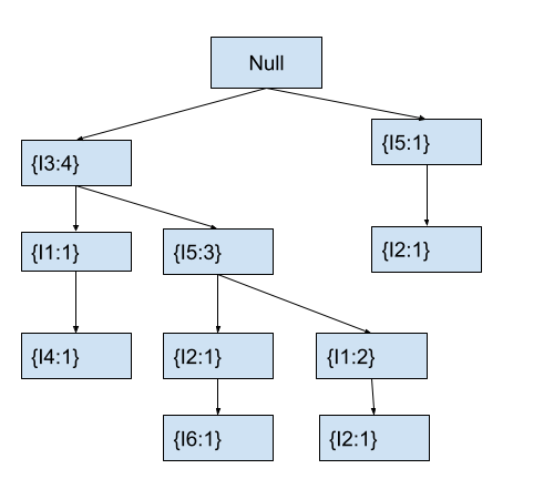
You might have difficulty understanding the above tree. In the next sections, we will discuss how to create an FP-Tree and how to interpret it. Then, you can easily interpret data from the above tree. Once we create an FP-Tree, we can generate frequent itemsets by recursively mining the tree. For this, we first create a pattern base for each frequent itemset using the fp-tree.

What is a Pattern Base in FP Growth Algorithm?

The pattern base in the FP-growth algorithm is a data structure that we use to store information about the conditional pattern bases for each frequent item in the dataset. We use a pattern base to capture the patterns or branches in the fp-tree that lead to a particular item. 

For each item in the frequent itemset, the pattern base records the set of transactions that contain the item, and the corresponding set of items in those transactions. For instance, the pattern base for item I1 in the fp-tree shown above will be [{I3}:1,{I3,I5}:2]. Here, we have denoted {I3} with count 1 because when we move from I3 to I1, the count associated with I1 is 1. Similarly, when we move from I3->I5->I1, the count associated with I1 is 2. Hence, the pattern is represented as {I3, I5}:2. 

After creating the pattern base for each frequent item in the transaction dataset, we create a conditional fp-tree for each item. 

What is the Conditional FP-Tree in FP Growth Algorithm?

The conditional fp-tree is a subset of the original FP-tree that only contains the transactions that contain a particular frequent item.

We construct the conditional FP-tree as part of the process of mining frequent patterns.  You can consider a conditional fp-tree for an item as an fp-tree constructed by first removing all items in the transaction dataset that are less frequent than the current item being considered. This is due to the reason that the less frequent items cannot be part of any frequent pattern that includes the current item. Why? 

Because we create the fp-tree by sorting the items in the transaction dataset using the support count of each item. Due to this, the nodes above a particular item in the fp-tree cannot have a support count lesser than the support count of the current item. The remaining transactions are then reorganized to form a new tree structure. Here, each node represents an item in the transactions and its frequency count. The new tree structure is then used as the conditional FP-tree for the current item.

For example, the conditional FP-Tree for item I1 will be as follows.

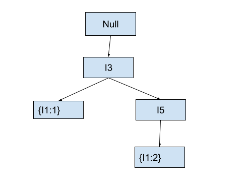
In the above conditional FP-Tree for item I1, you can conserve that I3 and I1 are present together in one transaction whereas items I3 and I5 are present together with I1 in two transactions. 

Till now, we have discussed all the data structures that we create in the fp growth algorithm. Let us now discuss a numerical example of the fp growth algorithm to understand all the steps in the algorithm in a better manner.

FP Growth Algorithm Numerical Example

As shown in the previous sections, we will use the following dataset to discuss the numerical example of the fp growth algorithm.

Transaction ID	Items
T1	I1, I3, I4
T2	I2, I3, I5, I6
T3	I1, I2, I3, I5
T4	I2, I5
T5	I1, I3, I5

The above dataset contains five transactions and 6 items. Now, let us discuss the fp growth algorithm step by step using the above dataset.

Step 1: Calculate The Support Count of Each Item in The Dataset

As a first step, we will first calculate the support count of all the items in the transaction dataset. The results have been tabulated below.

Item	Support Count
I1	3
I2	3
I3	4
I4	1
I5	4
I6	1

Now, let’s sort the above table by the support count. This will help us in the next step. The modified table looks as follows.

Item	Support Count
I3	4
I5	4
I1	3
I2	3
I4	1
I6	1

Step 2: Reorganize The Items in The Transaction Dataset

After calculating the support count of each item, we will sort the items in each transaction according to their support count in descending order. If two items have the same support count, we will keep their order in topological order. The resulting dataset is as follows.

Transaction ID	Items
T1	I3, I1, I4
T2	I3, I5, I2, I6
T3	I3, I5, I1, I2
T4	I5, I2
T5	I3, I5, I1

Step 3: Create FP Tree Using the Transaction Dataset

After sorting the items in each transaction in the dataset by their support count, we need to create an FP Tree using the dataset. 

To create an FP-Tree in the FP growth algorithm, we use the following steps.

1. First, we create a root node and name it Null or None. This node contains no data.
2. Now, for each transaction in the database, we insert the items in descending order of their support count into the FP-tree as follows:
   • First, we select a transaction containing items in descending order of their support count. Then, we go to the root node of the FP tree. We also select the first item of the current transaction.
   • Now, we check if any child node of the current node contains the current item in our transaction. If yes, we increment the support count of the item in the particular child node by 1 and move to that child node. We also move to the next item in the transaction.
   • If the current node doesn’t contain any child node with the current item in our transaction, we create a new child node with the current item and assign the count 1 to the item. Then, we move to the newly created child node. At the same time, we also move to the next item in the current transaction.
   • We follow the above steps for all the transactions in our dataset. 

After executing the above steps, we can create an fp-tree for any dataset. As the next step in our numerical example on the fp growth algorithm, let us create the fp-tree for our current dataset. 

Add Items from Transaction T1 to the FP Tree

First, we will create a Null node that represents the root of the fp tree. Then, we will select the first transaction with transaction T1 containing the sorted items [I3, I1, I4]. 

Currently, we are at the root node and the first item  I3 of the transaction T1. There is no child node of the current node that contains the item I3 (Of course the tree is empty right now.) Therefore, we will create a child node of the root node with item I3 and count 1. The tree looks as follows.

Now, we will move to the node I3 that we just created. We will also move to the next item I1 in the transaction. 

In the fp-tree, we will check if the current node has a child node with item I1. As the current node I3 has no child node with item I1, we will create a new node with item I1 and count 1. After this, the tree will look like this.

After creating the node with item I1, we will move to the newly created node. We will also move to the next item I4 in the current transaction. 

In the tree, we will check if any child node of the current node has item I4. In the fp-tree, the current node with item I1 has no child node with item I4. Hence, we will create a new node with item I4 and count 1 as a child node of the node containing I1. After this, the fp- tree will look as follows.

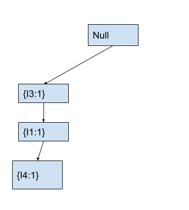
At this point, we have traversed all the items in transaction T1. Hence, we will move to transaction T2 containing items [I3, I5, I2, I6] and start a new iteration of the algorithm.

Add Items from Transaction T2 to the FP Tree

We start with item I3 at the root node. We first check if the current node contains any child node with the current item. As the child node of the root node already contains I3, we will increment the count of the child node containing I3 by 1. After this, the fp-tree looks as follows.

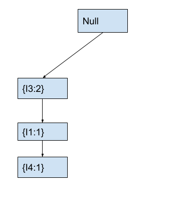
After creating the above tree, we will move to the node containing I3 that we modified. We will also move to the next item I5 in the current transaction T2. 

In the fp-tree, we will check if the current node has any child node with item I5. As the current node containing I3 has no child node with item I5, we will create a new node with item I5 and count 1 as a child of the node containing I3. After this, the fp- tree will look as follows.

Now, we will move to the node containing item I5 that we just created. We will also move to the next item I2 in the current transaction. 

In the fp-tree, the current node with item I5 has no child node with item I2. Hence, we will create a new child node with item I2 and count 1. After this, the fp tree will look as follows.

Next, we will move to node I2 that we just created. We will also move to the next item I6 in the current transaction. 

In the fp-tree, we will check if any child node of the current node contains item I6. The current node I2 has no child node with item I6. Hence, we will create a new child node with item I6 and count 1. After this, the fp tree will look like this.

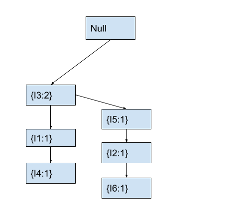
By now, we have completely traversed transaction T2. The above fp-tree represents the fp-tree for the transactions T1 and T2. Now, let us proceed to traverse transaction T3 containing items [I3, I5, I1, I2].

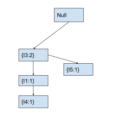
Add Items from Transaction T3 to the FP Tree

We start with item I3 at the root node. We first check if the current node contains any child node with the current item. As the child node of the root node already contains I3, we will increment the count of the child node containing I3 by 1. After this, the fp-tree looks as follows.

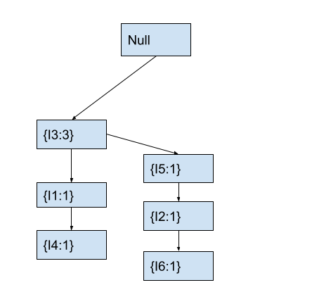
After creating the above tree, we will move to the node containing I3 that we modified. We will also move to the next item I5 in the current transaction. 

In the tree, the current node containing I3 already has a child node with item I5. Hence, we will increment the count of the child node I5 by 1. After this, the fp-tree looks as follows.

Now, we will move to node I5 that we just modified. We will also move to the next item I1 in the current transaction. 

In the tree, the current node I5 has no child node with item I1. Hence, we will create a new child node with item I1 and count 1. After this, the fp tree will look as follows.

Now, we will move to node I1 that we just created. We will also move to the next item I2 in the current transaction. 

In the tree, the current node I1 has no child node with item I2. Hence, we will create a new child node with item I2 and count 1. After this, the fp tree will look as follows.

At this point, we have traversed transaction T3. Hence, the above fp-tree represents the tree for transactions T1, T2, and T3. Now, we will traverse the transaction T4 with items [I5, I2]. 

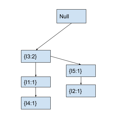
Add Items From Transaction T4 to the FP Tree

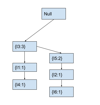
We start with item I5 at the root node. Here, we will first check if the current node contains any child node with the current item. As no child node of the root node contains I5, we will create a new child of the root node with item I5 and count 1. After this, the fp-tree looks as follows.

Now, we will move to node I5 that we just created. We will also move to the next item I2 in the current transaction. 

In the tree, the current node I5 has no child node with item I2. Hence, we will create a new child node with item I2 and count 1. After this, the fp tree will look as follows.

At this point, we have traversed transaction T4. Hence, the above fp-tree represents the tree for transactions T1, T2, T3, and T4. Now, we will traverse the transaction T5 with items [I3, I5, I1]. 

Add Items From Transaction T5 to the FP Tree

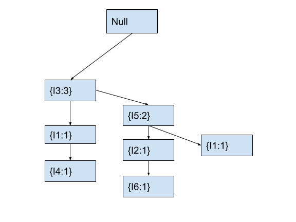
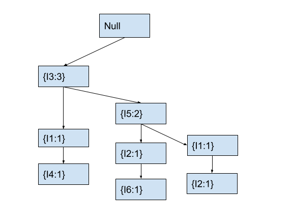
We start with item I3 at the root node. We first check if the current node contains any child node with the current item. As the child node of the root node already contains I3, we will increment the count of the child node containing I3 by 1. After this, the fp-tree looks as follows.

After creating the above tree, we will move to the node containing I3 that we just modified. We will also move to the next item I5 in the current transaction. 

In the tree, the current node containing I3 already has a child node with item I5. Hence, we will increment the count of the child node with item I5. After this, the fp- tree will look as follows.

Now, we will move to node I5 that we just modified. We will also move to the next item I1 in the current transaction. 

In the tree, the current node I5 already has a child node with item I1. Hence, we will increment the count of the child node with item I1 by 1. After this, the fp tree will look as follows.

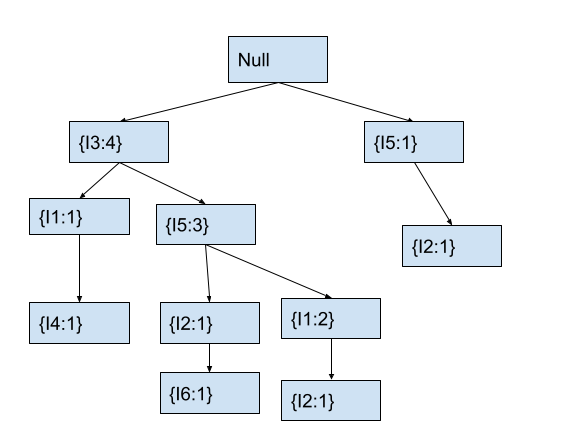
This is the final fp-tree created from all the transactions. Now, we will create a pattern base for all the frequent items in our dataset. For this, we will take the minimum support count of the items as 2.

Step 4: Create a Pattern Base For All The Items Using The FP-Tree

As the next step in our numerical example on the fp growth algorithm, we will create a pattern base for all the items in the transaction dataset. We have already discussed how to create a pattern base for an item using the fp-tree in the previous sections.

• The pattern base for item I1 in the fp-tree shown above will be [{I3}:1,{I3, I5}:2]. Here, we have denoted {I3} with count 1 because when we move from I3 to I1, the count associated with I1 is 1. Similarly, when we move from I3->I5->I1, the count associated with I1 is 2. Hence, the pattern is represented as {I3, I5}:2. 
• For item I2,  the pattern base will be [{I3,I5}:1,{I3,I5,I1}:1,{I5}:1]. Here, we have denoted {I3, I5} with count 1 because when we move from I3->I5->I2, the count associated with I2 is 1. Similarly, when we move from I3->I5->I1->I2, the count associated with I2 is 1. Hence, the pattern is represented as {I3, I5, I1}:1.  Next, when we move from I5->I2, the count of I2 is 1. Hence, the pattern is represented as {I5}:1.
• For item I3, there will be no pattern base as its directly connected to the root node.
• For item I5, when we move from I3->I5, the count for I5 is 3. Hence, the pattern base is  [{I3}:3]. 
• For items I4 and I6, there will be no pattern base as they do not have a support count greater than or equal to 2. Hence, they will not be included in the analysis.

The pattern base for each item in the dataset is tabulated below.

Item	Pattern Base
I1	{I3}:1,{I3, I5}:2
I2	{I3, I5}:1,{I3, I5, I1}:1,{I5}:1
I3	{}
I5	{I3}:3

Step 5: Create a Conditional FP Tree For Each Frequent Item

In the next step of this numerical example on fp growth algorithm, we will create a conditional fp-tree for each frequent item. I have already discussed what is a conditional fp-tree and how you can create it. Here, we will calculate the count of items in the conditional fp tree of each item.

• In the pattern base of item I1, item I3 comes in the pattern {I3} with count 1, and in the pattern {I3,I5} with count 2. Hence, the count of I3 in the conditional fp-tree of I1 will be 3. I5 only comes in the pattern {I3, I5}. Hence, its count in the conditional tree will be 2. The conditional fp-tree for item I1 will be {I3:3, I5:2}.
• For item I2, the pattern base contains I3 with a total count of 2, I5 with a total count of 3, and I1 with a total count of 1. As the count of I1 is less than the minimum support count, we will drop it. The conditional fp-tree for item I2 will be {I3:2, I5:3}.
• In the pattern base of item I5, I3 comes with count 3. Hence, the conditional fp-tree for I5 will be {I3:3}.

The conditional fp-tree for each item is tabulated below.

Item	Pattern Base	Conditional FP Tree
I1	{I3}:1,{I3, I5}:2	{I3:3, I5:2}
I2	{I3, I5}:1,{I3, I5, I1}:1,{I5}:1	{I3:2, I5:3}
I3	{}
I5	{I3}:3	{I3:3}

Step 6: Generate Frequent Itemsets From Conditional FP-Trees

After creating the conditional fp-tree, we will generate frequent itemsets for each item. To generate the frequent itemsets, we take all the combinations of the items in the conditional fp-tree with their count. For instance,

• The frequent itemsets from the conditional fp-tree of item I1 will be [{I1, I3}:3,{I1, I5}:2,{I1, I3, I5}:2]. Here, the support count of the itemset {I1, I3} is 3 as the maximum support count of I3 in the conditional fp-tree is 3. Similarly, the support count of the itemset {I1, I5} is 2  as the maximum support count of I5 in the conditional fp-tree is 2. Finally, the support count of {I1, I3, I5} is 2 as I5 restricts the itemset from having more support count as it has a support count of only 2.
• Frequent itemsets from the conditional fp-tree of item I2 will be [{I2, I3}:2,{I2, I5}:3,{I2, I3, I5}:2]. Here, the support count of the itemset {I2, I3} is 2 as the maximum support count of I3 in the conditional fp-tree is 2. Similarly, the support count of the itemset {I2, I5} is 3  as the maximum support count of I5 in the conditional fp-tree is 3. Finally, the support count of {I2, I3, I5} is 2 as I3 restricts the itemset from having more support count as it has a support count of only 2.
• We can get only one frequent itemset from the conditional fp-tree of I5 i.e. {I3, I5} with count 3.

All the frequent itemsets derived from the conditional fp-trees have been tabulated below.

Item	Pattern Base	Conditional FP Tree	Frequent itemsets
I1	{I3}:1,{I3, I5}:2	{I3:3, I5:2}	{I1, I3}:3,{I1, I5}:2,{I1, I3, I5}:2
I2	{I3, I5}:1,{I3, I5, I1}:1,{I5}:1	{I3:2, I5:3}	{I2, I3}:2, {I2, I5}:3,{I2, I3, I5}:2
I5	{I3}:3	{I3:3}	{I3, I5}:3

Step 7: Generate Association Rules

After obtaining the frequent itemsets, we can generate association rules. I have already explained how to create association rules from the above frequent itemsets at this link.

Conclusion

In this article, we discussed the fp growth algorithm with a numerical example. To learn more about data mining and machine learning, you can read this article on k-means clustering numerical example. You might also like this article on KNN classification numerical example.

I hope you enjoyed reading this article. Stay tuned for more informative articles!

Happy Learning!