Implement Apriori Algorithm in Python

We use different algorithms to perform market basket analysis in data mining. For this, we use the apriori algorithm, fp-growth algorithm, and the ECLAT algorithm to find frequent item sets and association rules. This article will discuss how to implement the apriori algorithm in Python.

How to Implement Apriori Algorithm in Python?

To implement the apriori algorithm in Python, we will use the mlxtend module. If you haven’t read the basics of the apriori algorithm, I would suggest you first read this article on the apriori algorithm numerical example.

For implementing the apriori algorithm in Python, we will use the following steps. 

• We will first obtain the transaction dataset in a list of lists.
• Next, we will create the transaction array using one-hot encoding with the TransactionEncoder() function. 
• Once we get the transaction array, we will calculate the frequent itemsets using the apriori() function defined in the mlxtend module in Python. 
• Finally, we will perform association rule mining using the association_rules() function from the mlxtend module.

Generate Transaction Array Using One Hot Encoding

To implement the apriori algorithm in Python, we will use the following dataset.

Transaction ID	Items
T1	I1, I3, I4
T2	I2, I3, I5, I6
T3	I1, I2, I3, I5
T4	I2, I5
T5	I1, I3, I5

The above transaction dataset contains 5 transactions with six distinct items. From the above table, we will create a list of lists of the items in the transactions as shown below.

transactions=[["I1", "I3", "I4"],
             ["I2", "I3", "I5", "I6"],
             ["I1", "I2", "I3", "I5"],
             ["I2", "I5"],
             ["I1", "I3", "I5"]]

Now, we will convert the transaction data into an array of transactions and items. The array has the following properties.

• Each row in the array represents a transaction and each column represents an item.
• Each element in the array is set to True or False.
• If an item is present in a particular transaction, the element at the corresponding row and column will be set to True.
• If an item isn’t present in a transaction, the element corresponding to the particular row and column is set to False. 

To generate the transaction array, we will use the TransactionEncoder() function defined in the mlxtend module. The TransactionEncoder() function returns a TransactionEncoder object. 

• We can use the TransactionEncoder object to array format suitable for typical machine learning APIs. For this, we will use the fit() and transform() methods. 
• The fit() method takes the transaction data in the form of a Python list of lists. Then, the TransactionEncoder object learns all the unique labels in the dataset.
• Next, we will use the transform() method to transform the input dataset into a one-hot encoded NumPy boolean array as shown below.

from mlxtend.preprocessing import TransactionEncoder
transactions=[["I1", "I3", "I4"],
             ["I2", "I3", "I5", "I6"],
             ["I1", "I2", "I3", "I5"],
             ["I2", "I5"],
             ["I1", "I3", "I5"]]
print("The list of transactions is:")
print(transactions)
transaction_encoder = TransactionEncoder()
transaction_array = te.fit(transactions).transform(transactions)
print("The transaction array is:")
print(transaction_array)

Output:

The list of transactions is:
[['I1', 'I3', 'I4'], ['I2', 'I3', 'I5', 'I6'], ['I1', 'I2', 'I3', 'I5'], ['I2', 'I5'], ['I1', 'I3', 'I5']]
The transaction array is:
[[ True False  True  True False False]
 [False  True  True False  True  True]
 [ True  True  True False  True False]
 [False  True False False  True False]
 [ True False  True False  True False]]

By default, the transform() method creates a boolean array containing the True and False values. If you want to create an array of 0s and 1s, you can use the astype() method.

The astype() method, when invoked on a numpy array, takes a data type as its input argument and converts the array elements to the desired data type. When we convert the array of boolean values to integer, True values will be converted to 1s and False values will be converted to 0s.

You can observe this in the following example.

from mlxtend.preprocessing import TransactionEncoder
transactions=[["I1", "I3", "I4"],
             ["I2", "I3", "I5", "I6"],
             ["I1", "I2", "I3", "I5"],
             ["I2", "I5"],
             ["I1", "I3", "I5"]]
print("The list of transactions is:")
print(transactions)
transaction_encoder = TransactionEncoder()
transaction_array = transaction_encoder.fit(transactions).transform(transactions).astype("int")
print("The transaction array is:")
print(transaction_array)

Output:

The list of transactions is:
[['I1', 'I3', 'I4'], ['I2', 'I3', 'I5', 'I6'], ['I1', 'I2', 'I3', 'I5'], ['I2', 'I5'], ['I1', 'I3', 'I5']]
The transaction array is:
[[1 0 1 1 0 0]
 [0 1 1 0 1 1]
 [1 1 1 0 1 0]
 [0 1 0 0 1 0]
 [1 0 1 0 1 0]]

The array of boolean values has better performance than the array of integer values. So, we will use the transaction array containing boolean values to implement the apriori algorithm in Python.

For better visualization, we will convert the array into a dataframe using the DataFrame() function defined in the pandas module in Python. Here, we will set the item names as the column names in the dataframe. You can obtain all the item names using the columns_ attribute of the TransactionEncoder object as shown below.

from mlxtend.preprocessing import TransactionEncoder
import pandas as pd
transactions=[["I1", "I3", "I4"],
             ["I2", "I3", "I5", "I6"],
             ["I1", "I2", "I3", "I5"],
             ["I2", "I5"],
             ["I1", "I3", "I5"]]
transaction_encoder = TransactionEncoder()
transaction_array = transaction_encoder.fit(transactions).transform(transactions)
transaction_dataframe = pd.DataFrame(transaction_array, columns=transaction_encoder.columns_)
print("The transaction dataframe is:")
print(transaction_dataframe)

Output:

The transaction dataframe is:
      I1     I2     I3     I4     I5     I6
0   True  False   True   True  False  False
1  False   True   True  False   True   True
2   True   True   True  False   True  False
3  False   True  False  False   True  False
4   True  False   True  False   True  False

Generate Frequent Itemsets Using The apriori() Function

Now that we have obtained the transaction array as a pandas dataframe, we will generate all the frequent itemsets. For this, we will use the apriori algorithm. The mlxtend module provides us with the apriori() function to implement the apriori algorithm in Python. It has the following syntax. 

apriori(df, min_support=0.5, use_colnames=False, max_len=None, verbose=0, low_memory=False)

Here, 

• df is the dataframe created from the transaction matrix. 
• min_support is the minimum support that we want to specify. It should be a floating point number between 0 and 1. The support is computed as the ratio of the number of transactions where a particular item set occurs to the total number of transactions.
• The use_colnames parameter is used to specify if we want to use the column names of the input df as the item names. By default, use_colnames is set to False. Due to this, the apriori() function uses the index of the columns instead of the column names as item names. To use the column names of the input df as item names, you can set the use_colnames parameter to True.
• The max_len parameter is used to define the maximum number of items in an itemset. By default, it is set to None denoting that all possible itemsets lengths under the apriori condition are evaluated.
• The low_memory parameter is used to specify if we have resource constraints. If we set the low_memory parameter to True, the apriori algorithm uses an iterator to search for combinations above min_support. You should only set low_memory=True for large datasets if memory resources are limited. When the low_memory parameter is set to True, the execution of the apriori algorithm becomes approx. 3-6x slower than the default value to optimize for the memory.
• The verbose parameter is used to show the execution stage for the apriori algorithm in Python. You can set the verbose parameter to a value greater than 1 to show the number of iterations when the low_memory parameter is True.  When the verbose parameter is set to 1 and low_memory is set to False, the function shows the number of combinations while executing the apriori algorithm in python.

After execution of the apriori() function,  we will get a pandas DataFrame with columns ['support', 'itemsets'] of all itemsets that have the support greater than or equal to the min_support and length less than max_len if max_len is not None. Each itemset in the ‘itemsets‘ column is of type frozenset, which is a Python built-in type that behaves similarly to sets except that it is immutable

To calculate the frequent itemsets, we will use a support of 0.4 and set the use_colnames parameter to True to use the column names of the input dataframe as item names.

You can observe this in the following example.

from mlxtend.preprocessing import TransactionEncoder
from mlxtend.frequent_patterns import apriori
import pandas as pd
transactions=[["I1", "I3", "I4"],
             ["I2", "I3", "I5", "I6"],
             ["I1", "I2", "I3", "I5"],
             ["I2", "I5"],
             ["I1", "I3", "I5"]]
transaction_encoder = TransactionEncoder()
transaction_array = transaction_encoder.fit(transactions).transform(transactions)
transaction_dataframe = pd.DataFrame(transaction_array, columns=transaction_encoder.columns_)
freuent_itemsets=apriori(transaction_dataframe,min_support=0.4, use_colnames=True)
print("The frequent itemsets are:")
print(freuent_itemsets)

Output:

The frequent itemsets are:
    support      itemsets
0       0.6          (I1)
1       0.6          (I2)
2       0.8          (I3)
3       0.8          (I5)
4       0.6      (I1, I3)
5       0.4      (I1, I5)
6       0.4      (I2, I3)
7       0.6      (I2, I5)
8       0.6      (I3, I5)
9       0.4  (I1, I3, I5)
10      0.4  (I2, I3, I5)

Generate Association Rules Using The association_rules() Function

After generating the frequent itemsets, we will calculate the association rules. For this, we will use the association_rules() function defined in the mlxtend module in Python. The association_rules() function has the following syntax.

association_rules(df, metric='confidence', min_threshold=0.8, support_only=False)

Here, 

• df is the dataframe returned from the apriori() function. It must contain the columns 'support‘ and ‘itemsets‘ containing frequent itemsets and their support.
• The metric parameter defines the metric used to select the association rules. The association_rules() function supports the following metrics.
  • “support”: The support for an association rule is calculated as the sum of support of the antecedent and the consequent. It has a range of [0,1].
  • “confidence”: The confidence of an association rule is calculated as the support of the antecedent and consequent combined divided by the support of the antecedent.  It has a range of [0,1].
  • “lift”: The lift for an association rule is defined as the confidence of the association rule divided by the support of the consequent. It has a range of [0, infinity].
  • “leverage”: The leverage of an association rule is defined as the ratio of support of the association rule to the product of support of antecedent and consequent. It has a range of [-1,1].
  • “conviction”: The conviction of an association rule is defined as (1-support of consequent) divided by (1- confidence of the association rule). It has a range of [0, infinity].
  • “zhangs_metric”: It is calculated as leverage of the association rule/max (support of the association rule*(1-support of the antecedent), support of the antecedent*(support of the consequent-support of the association rule)). It has a range of [-1,1].
• The min_threshold parameter takes the minimum value of the metric defined in the metric parameter to filter the useful association rules. By default, it has a value of 0.8.
• The support_only parameter is used to specify if we only want to compute the support of the association rules and fill the other metric columns with NaNs. You can use this parameter if the input dataframe is incomplete and does not contain support values for all rule antecedents and consequents. By setting the support_only parameter to True, you can also speed up the computation because you don’t calculate the other metrics for the association rules.

After execution, the association_rules() function returns a dataframe containing the ‘antecedents’, ‘consequents’, ‘antecedent support’, ‘consequent support’, ‘support’, ‘confidence’, ‘lift’, ‘leverage’, and ‘conviction’ for all the generated association rules.

You can observe this in the following example.

from mlxtend.preprocessing import TransactionEncoder
from mlxtend.frequent_patterns import apriori, association_rules
import pandas as pd
transactions=[["I1", "I3", "I4"],
             ["I2", "I3", "I5", "I6"],
             ["I1", "I2", "I3", "I5"],
             ["I2", "I5"],
             ["I1", "I3", "I5"]]
transaction_encoder = TransactionEncoder()
transaction_array = transaction_encoder.fit(transactions).transform(transactions)
transaction_dataframe = pd.DataFrame(transaction_array, columns=transaction_encoder.columns_)
freuent_itemsets=apriori(transaction_dataframe,min_support=0.4, use_colnames=True)
association_rules_df=association_rules(freuent_itemsets, metric="confidence", min_threshold=.75)
print("The association rules are:")
print(association_rules_df)

Output:

The association rules are:
  antecedents consequents  antecedent support  consequent support  support  \
0        (I1)        (I3)                 0.6                 0.8      0.6   
1        (I2)        (I5)                 0.6                 0.8      0.6   
2    (I1, I5)        (I3)                 0.4                 0.8      0.4   
3    (I2, I3)        (I5)                 0.4                 0.8      0.4   

   confidence  lift  leverage  conviction  
0         1.0  1.25      0.12         inf  
1         1.0  1.25      0.12         inf  
2         1.0  1.25      0.08         inf  
3         1.0  1.25      0.08         inf  

Complete Implementation of the Apriori Algorithm in Python

In the previous sections, we have discussed how to implement the apriori algorithm in Python using the functions defined in the mlxtend module and a dummy dataset. Now, let us discuss how to implement the apriori algorithm in Python on a real-world dataset. 

Consider that we have a transaction dataset given at this link. You can download the dataset to implement the program. 

Load and Pre-Process The Dataset

To load the dataset, we will use the read_csv() method defined in the pandas module in Python. It returns a dataframe as shown below.

import pandas as pd
dataset=pd.read_csv("ecommerce_transaction_dataset.csv")
dataset.head()

Output:

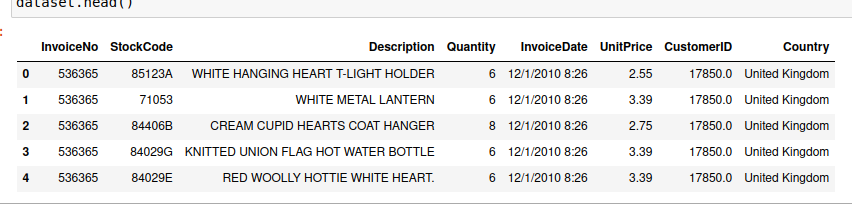
In the above data, we only need the transaction id ie. “InvoiceNo” and item id i.e. “StockCode” columns. Hence, we will select these columns. Also, we will drop the rows in which transaction id or item ids are null values.

import pandas as pd
dataset=pd.read_csv("ecommerce_transaction_dataset.csv")
dataset=dataset[["InvoiceNo","StockCode"]]
dataset=dataset.dropna()
dataset.head()

Output:

	InvoiceNo StockCode
0 	536365 	85123A
1 	536365 	71053
2 	536365 	84406B
3 	536365 	84029G
4 	536365 	84029E

In the above output, you can observe that each row contains only one item. Hence, we will group all the items of a particular transaction in a single row. For this, we will use the groupby() method, the apply() method, and the list() function.

• The groupby() method, when invoked on a dataframe, takes the column name i.e. “InvoiceNo” as its input argument. After execution, it groups the rows for a particular InvoiceNo into small dataframes. 
• Next, we will make a list of all items in the transaction by applying the list() function on the  “StockCode” column of each grouped dataframe using the apply() method.

After executing the above methods, we will get a dataframe containing the transaction id and the corresponding items as shown below.

import pandas as pd
dataset=pd.read_csv("ecommerce_transaction_dataset.csv")
dataset=dataset[["InvoiceNo","StockCode"]]
dataset=dataset.dropna()
transaction_data=dataset.groupby("InvoiceNo")["StockCode"].apply(list).reset_index(name='Items')
transaction_data.head()

Output:

  InvoiceNo                                              Items
0    536365  [85123A, 71053, 84406B, 84029G, 84029E, 22752,...
1    536366                                     [22633, 22632]
2    536367  [84879, 22745, 22748, 22749, 22310, 84969, 226...
3    536368                       [22960, 22913, 22912, 22914]
4    536369                                            [21756]

Now, we will select the StockCode column to make a list of lists of items in the transactions as shown below.

import pandas as pd
dataset=pd.read_csv("ecommerce_transaction_dataset.csv")
dataset=dataset[["InvoiceNo","StockCode"]]
dataset=dataset.dropna()
transaction_data=dataset.groupby("InvoiceNo")["StockCode"].apply(list).reset_index(name='Items')
transactions=transaction_data["Items"].tolist()

Implement the Apriori Algorithm on The Processed Data

Once we get the list of lists of all the items after data preprocessing, we can use the apriori() function to implement the apriori algorithm in Python as shown below.

from mlxtend.preprocessing import TransactionEncoder
from mlxtend.frequent_patterns import apriori, association_rules
import pandas as pd
import pandas as pd
dataset=pd.read_csv("ecommerce_transaction_dataset.csv")
dataset=dataset[["InvoiceNo","StockCode"]]
dataset=dataset.dropna()
transaction_data=dataset.groupby("InvoiceNo")["StockCode"].apply(list).reset_index(name='Items')
transactions=transaction_data["Items"].tolist()
transaction_encoder = TransactionEncoder()
transaction_array = transaction_encoder.fit(transactions).transform(transactions)
transaction_dataframe = pd.DataFrame(transaction_array, columns=transaction_encoder.columns_)
freuent_itemsets=apriori(transaction_dataframe,min_support=0.02, use_colnames=True)
print("The frequent itemsets are:")
print(freuent_itemsets)

Output:

The frequent itemsets are:
      support               itemsets
0    0.020193                (15036)
1    0.027181                (20685)
2    0.020541                (20711)
3    0.033668                (20712)
4    0.026023                (20713)
..        ...                    ...
215  0.022471        (23203, 85099B)
216  0.021197         (23300, 23301)
217  0.022896       (85099B, 85099C)
218  0.021042       (85099B, 85099F)
219  0.021197  (22699, 22698, 22697)

[220 rows x 2 columns]

You can also calculate the association rules using the association_rules() function as shown below.

from mlxtend.preprocessing import TransactionEncoder
from mlxtend.frequent_patterns import apriori, association_rules
import pandas as pd
import pandas as pd
dataset=pd.read_csv("ecommerce_transaction_dataset.csv")
dataset=dataset[["InvoiceNo","StockCode"]]
dataset=dataset.dropna()
transaction_data=dataset.groupby("InvoiceNo")["StockCode"].apply(list).reset_index(name='Items')
transactions=transaction_data["Items"].tolist()
transaction_encoder = TransactionEncoder()
transaction_array = transaction_encoder.fit(transactions).transform(transactions)
transaction_dataframe = pd.DataFrame(transaction_array, columns=transaction_encoder.columns_)
freuent_itemsets=apriori(transaction_dataframe,min_support=0.02, use_colnames=True)
association_rules_df=association_rules(freuent_itemsets, metric="confidence", min_threshold=.50)
print("The association rules are:")
print(association_rules_df.head())

Output:

The association rules are:
  antecedents consequents  antecedent support  consequent support   support  \
0     (20712)    (85099B)            0.033668            0.082432  0.020772   
1     (22356)     (20724)            0.029344            0.040541  0.020309   
2     (20724)     (22356)            0.040541            0.029344  0.020309   
3     (20726)     (20725)            0.040039            0.062085  0.020541   
4     (20727)     (20725)            0.050000            0.062085  0.025019   

   confidence       lift  leverage  conviction  
0    0.616972   7.484584  0.017997    2.395566  
1    0.692105  17.071930  0.019119    3.116193  
2    0.500952  17.071930  0.019119    1.945018  
3    0.513018   8.263168  0.018055    1.925976  
4    0.500386   8.059701  0.021915    1.877280  

Conclusion

In this article, we discussed how to implement the apriori algorithm using the mlxtend module in Python. To know more about data mining concepts, you can read this article on the fp-growth algorithm numerical example. You might also like this article on the ECLAT algorithm numerical example.

I hope you enjoyed reading this article. Stay tuned for more informative articles. 

Happy Learning!